
Fitting
I went back and looked at the data in my Network Dispersion post from a while ago. At the time I didn't plot it to show the strong power-law characteristics of the dispersive rate formulation, so replotted it here:
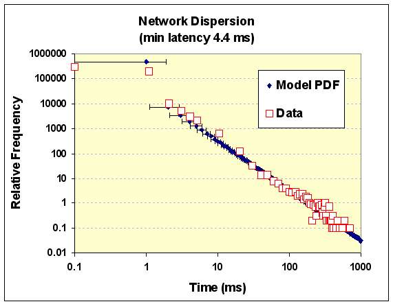
This is a simple distributed latency caused by the dispersed network transport rate, where the cumulative P(Time) = exp(-T0/Time). The derivative is a PDF and this gives the 1/Time2 slope shown (adjusted for the log density along the horizontal axis). Some uncertainty exists in the minimum measurable round-trip time at around 1 ms, but the rest of the curve agrees with the simple entropic dispersion -- a slight variation of the basic entroplet in action.
Neater still is the entropic dispersion in daily rainfall data. I happened across research work at the National Center for Atmospheric Research under the title "Extreme Event Density Estimation". The researchers there seem to think the following graph has some mysterious structure. It basically displays a histogram of daily rainfall in January at a station in North Carolina.
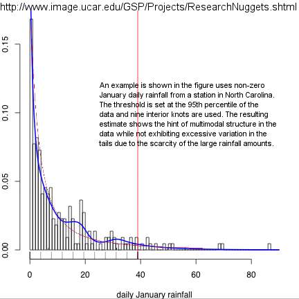
On first glance, this data doesn't appear highly dispersed as the tail stays fairly thin, yet take a look at this fit:

You need to understand first that a critical point exists for rain to fall. The volume and density at which nature reaches this critical point has much to do with the rate at which a cloud increases in intensity. If we assume that clouds develop by some sort of preferential attachment, then the uncertainties at which the preferential attachment process increases with time balanced against the uncertainties in the critical point contribute to the entropic dispersion:
p(x) = r/(r+g(x))2The term g(x) essentially measures the preferential attachment accelerated growth rate:
g(x) = k*(exp(a*x) - 1)This has the mechanism for preferential attachment since dg/dx = a * (g(x)+k), which describes exponential growth plus a linear term. When plotted, we get the orange curve shown plotted along with the data points, where r=1, a=1/17 years and k=2 (dimensions in mm). Coicidentally, this is actually just the logistic sigmoid function; we never see the characteristic peak or inflection point since it starts off well up the towards the halfway point of the cumulative (see the following graph where I used r=10 to accentuate the sigmoid peak).

In spite of the good fit, this curve has a limited locality: consisting of one rainfall station in North Carolina. What happens when we look at the distribution of rainfall on a global scale?
This poster and slide show attempts an understanding of the distribution via entropy arguments.
The curve below does not work as well for the exponential growth (bright green) but it does work very well for the cubic-quadratic growth model (cumulative growth ~ x5, bright turquoise) that I used in my analysis of dispersive discovery of oil reservoirs. (note that this curve is plotted in hydrologist's lingo, where the rate of return in years T equates to a histogram bin. The rate of return analogizes to principle such as the "100 year storm"). The values shown here are in inches of rainfall, not millimeters as in the previous figure.
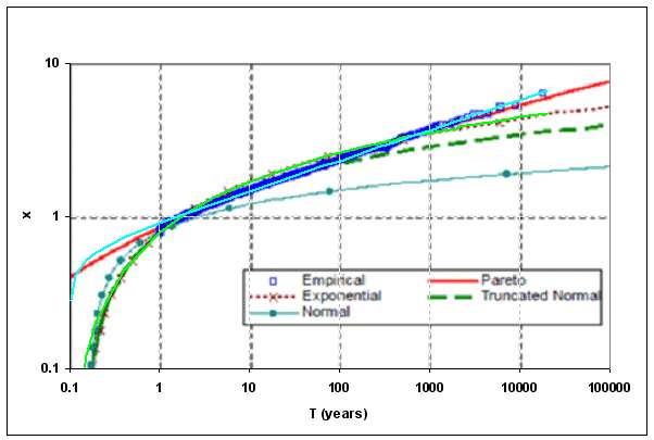
Since we can expand an exponential in terms of a Taylor series and see a sum of power terms, it makes some sense that the t 5 term may emulate the exponential growth (or vice versa), or perhaps generate the limiting trend. Exponential growth eventually moderates and the 5th power may provide the major effect along the curve over the remainder of the fat tail (note that the power is 5 and not 6 in the cubic-quadratic model because rainfall is measured as a linear measure and growth of water content goes as volumetric density).
As the arguments for oil discovery (uncertain acceleration in technology along an uncertain volume) emulate rain strength (uncertain acceleration in cloud/droplet growth along an uncertain critical volume/density), I consider this a further substantiation of the overall entropic dispersion formulation.
Yet I've got to wonder: do climate scientists think this way? The hydrology researcher Koutsoyiannis, who identified the power-law dependence in the previous figure, seems to have gotten on the right track. His multiple Markov chain remains a bit unwieldy as he can only generate a profile via simulation, yet that may not matter if we can use a power-law argument directly as I did for dispersive discovery. This needs a deeper look as it exposes a few remaining modeling details in a comprehensive theory.
Speaking of odd, why do these rather simple arguments always seem to work so well, and, extending that, could dispersion work everywhere? The odd thing is that the odds function may hold a bit of the key. Everyone seems to understand how gambling works, particularly in the form of sports betting, where just about any lame-brained man-off-the-street comprehends how the odds function works. Odds against for some competitor to win is essentially cast in terms of the probability P:
Odds = (1-P)/PWhen plotted the odds distribution looks like the following curve:

Which then looks exactly like the rank histogram of any scaled entropic dispersion process:

So we can give the odds of discovering a size of a certain reservoir in comparison to the median characteristic value just by taking the ratio between the two values. This equates well to the relative payout of somebody who beat the odds and beat the house. Pretty simple.
As a provocative statement, we do understand this all too well, because if we can understand gambling, then we should understand the math behind dispersion. What likely gets in the way is the math itself. People have a math phobia in that as long as they don't know that they need to invoke math, they feel confident. So the odds function becomes perfectly acceptable, as it has some learned intuition behind it. As Jaynes would suggest, this has become part of our Bayesian conditioned belief system. Enough processes obey the dispersive effect that it becomes second nature to us -- if we deal with it on a sub-conscious level.
The odds-makers don't really have to think, they just make sure that the cumulative probability sums to one over the rank histogram. Then, since the pay-outs will balance out in some largely predictable fashion, they can remain confident that they won't get left holding the bag. Why can't the oil punditocracy make the same sense to our oil predictions, I only have a hunch.
PostEdit:
Here is a graph of an exponential morphing into a x^6 dependence by limiting the Taylor series expansion of the exponential to 6 terms.

posted by @whut at March 25, 2010
![]()
![]()


0 Comments:
Post a Comment
<< Home