Oil Discovery Simulation Reality

I should have run this particular simulation long ago. In this exercise, I essentially partitioned the Dispersive Discovery model into a bunch of subvolumes. Each subvolume belongs to a specific prospecting entity, which I have given a short alias. The simulation assigns each one of the entities a random search rate and each one of the subvolumes also has a randomly sized value. The physical analogy equates to the prospector (i.e. the entity is an owner, leaser, company, nation, etc.) given their own subvolume (geographic location) to explore for oil. When they exhaustively search that subvolume, they end up with a cumulative amount of oil. The abstraction for subvolumes allows for the random sizing to directly translate to a proportional amount of oil. In general, bigger subvolumes equates to more oil but this does not have to hold, since the random rates blur this distinction.

Removing the technical mumbo-jumbo, the previous paragraph describes quite simply the context for the dispersive discovery model. Nothing about this description can possibly get misinterpreted as it essentially describes the process of a bunch of people systematically searching through a haystack for needles. Each person has varying ability and owns a varying size to search through, which essentially describes the process of dispersion.

The random number distributions derive from a mean search rate and a mean subvolume based on the principle of maximum entropy (MaxEnt). The number of subvolumes multiplied by the mean subvolume generates an ultimately recoverable resource (URR) total. By building a Monte Carlo simulation of this model, we can see how the discovery process plays out for randomly chosen configurations.

When the simulation executes, the search rates accelerate in unison so that the variance remains the same, maintaining MaxEnt of the aggregate. If I choose an exponential acceleration, the result turns precisely into the Logistic sigmoid, also known as the classic Hubbert Curve..

The entire simulation exists on a Google spreadsheet. Each row corresponds to a prospecting entity/subvolume pairing. The first two cells provide a random starting rate and a randomly assigned subvolume. As you move left to right across the row, you see the fraction of the subvolume searched increase in an accelerating fashion with respect to time. The exponential growth factor resides in cell A2. At some point in time, the accelerating search volume meets the fixed volume constraint and the number stops increasing. At that moment, the prospector has effectively finished his search. That subvolume has essentially ceased to yield newly discovered oil.

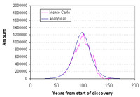
I reserve the 4th row for the summed values, the 3rd line generates the time derivative which plots out as a yearly discovery. The simulation "runs" one Monte Carlo frame at a time. We essentially see a full snapshot of one sample for about 150 years of dispersive search.

View Google Spreadsheet

I associated short names for each of the prospecting entities[1]. As I did not to want to make the spreadsheet too large, I limited it to 250 entities (which pushes Google to the limit for data). This of course introduces some noise fluctuations. The non-noisy solid line displays the analytical solution to the dispersive discovery model, which happens to match the derivative of the Logistic sigmoid.

The most important insight that we get from this exercise has to do with generating a BLINDINGLY SIMPLE explanation for deriving the Logistic behavior that most oil depletion analysts assume to exist, yet have no basis for. For crying out loud, I have seen children's board games with more complicated instructions than what I have given in the above paragraphs. Honestly, if you find someone that can't understand what it is going on from what I have written, don't ask them to play Chutes & Ladders either. Common sense Peak Oil theory ultimately reduces to this basic argument.

Contrast the elegance of the dispersive model with the most common alternative derivation for the logistic peak shape. This involves a completely misguided deterministic model that not surprisingly makes ABSOLUTELY NO SENSE. Whoever originally dreamed up the Verhulst derivation for ecological modeling and decided to apply it to Peak Oil must have consumed large quantities of mind-altering drugs prior to putting pencil to paper.

I also want to point out that what I did has nothing to do with multi-cycle Hubbert modeling which adds even less insight to the fundamental process.

I hope that this exercise helps in understanding the mechanism behind dispersive discovery. Seriously, the big intuitive sticking point that people have with the model has to do with the lack of any feedback mechanism in dispersive discovery. I imagine that engineers and most scientists get so used to seeing the feedback-derived Verhulst and LV equations derive the Logistic that they can't believe a simple and correct formulation actually exists!

In real terms, at some point the oil companies will cease to discover much of anything as they exhaust search possibilities. I suggest that they might want to consider making up for lost profit by licensing the oil discovery board game. This would help explain to their customers the reality of the situation.

UPDATE:
Occasionally Google does an underflow or overflow on some calculations so that the aggregate curve won't plot. The following animated GIF shows a succession of curves:

---

[1] I used shortened versions of TOD commenter names in the spreadsheet to make it a little more entertaining. I probably spent more time on writing the names down and battling the sluggishness of Google spreadsheet than I did on the simulation.